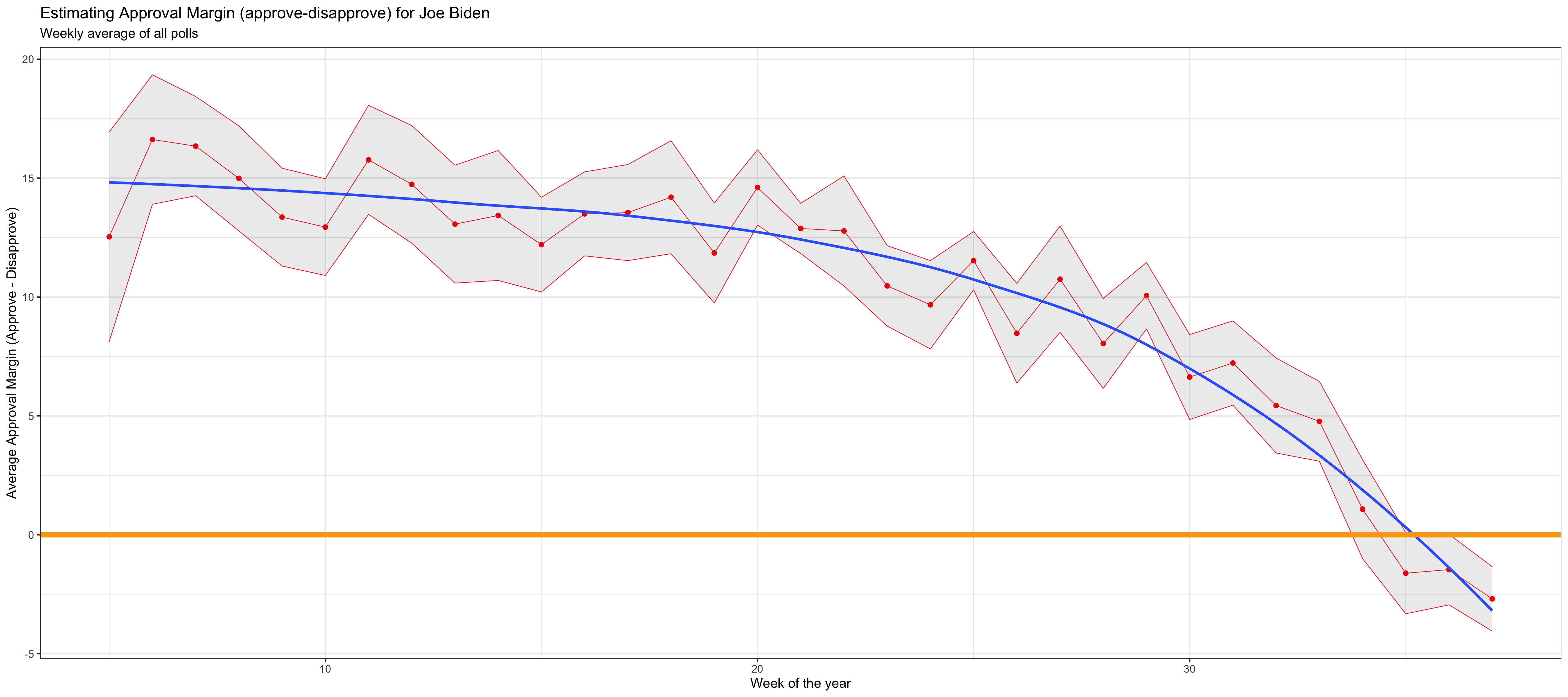
Biden's Approval Margin
plot <- approval_polllist %>%
  mutate(week=week(enddate)) %>% #Creating a new column called week by extracting the week from the enddate variable
  group_by(week) %>%
  mutate(
    net_approval_rate=approve-disapprove #Creating a new column called net_approval_rate by subtracting disapprove from approve
  ) %>%
  summarise(
    mean=mean(net_approval_rate), #Mean net approval by week
    sd=sd(net_approval_rate), #Standard deviation of net approval by week
    count=n(), #Count by week
    se=sd/sqrt(count), #Standard error of the week
    t_critical=qt(0.975, count-1), #T-critical value
    lower=mean-t_critical*se, #Lower end of the CI
    upper=mean+t_critical*se #Upper end of the CI
  ) %>%

  #Scatterplot of the calculated net approval rate means by week
  ggplot(aes(x=week, y=mean)) +
  geom_point(colour='red') + #Scatterplot using red points
  geom_line(colour='red', size=0.25) + #Adding a red line to connect the points
  geom_ribbon(aes(ymin=lower, ymax=upper), colour='red', linetype=1, alpha=0.1, size=0.25) +
  geom_smooth(se=F) + #Adding a smooth line for the trend
  geom_hline(yintercept=0, color='orange', size=2) + #Adding an orange horizontal line
  theme_bw() + #Theme
  labs(title='Estimating Approval Margin (approve-disapprove) for Joe Biden', #Adding a title
       subtitle='Weekly average of all polls', #Subtitle
       x='Week of the year', #X-label
       y='Average Approval Margin (Approve - Disapprove)') + #Y-label
  NULL

ggsave(file='bidenplot_home.jpg', plot=plot, path = '~/Desktop/LBS/Term1/my-website/my-website/static/img', height=18, width = 18)

ggsave(file='bidenplot.jpg', plot=plot, path = '~/Desktop/LBS/Term1/my-website/my-website/static/img', height=8, width = 18)