GDP Components
Data Cleaning
#Creating a new data set after converting to the long format, transforming the figure to billions, and simplifying the indicator names

tidy_GDP_data  <-  UN_GDP_data %>%
  pivot_longer(cols = 4:51, names_to = 'Year', values_to = 'Value') %>%
  mutate(
    Value = Value/1e9,
    IndicatorName = case_when(
      IndicatorName == "Household consumption expenditure (including Non-profit institutions serving households)" ~ "Household expenditure",
      IndicatorName == "General government final consumption expenditure" ~ "Government expenditure",
      IndicatorName == "Gross fixed capital formation (including Acquisitions less disposals of valuables" ~"Gross fixed capital formation",
      IndicatorName == "Exports of goods and services" ~ "Exports",
      IndicatorName == "Imports of goods and services" ~ "Imports",
      IndicatorName == "Gross Domestic Product (GDP)" ~ "GDP",
      IndicatorName == "Agriculture, hunting, forestry, fishing (ISIC A-B)" ~ "AHFF",
      IndicatorName == "Mining, Manufacturing, Utilities (ISIC C-E)" ~ "MMU",
      IndicatorName == "Manufacturing (ISIC D)" ~ "Manu",
      IndicatorName == "Construction (ISIC F)" ~ "Cons",
      IndicatorName == "Wholesale, retail trade, restaurants and hotels (ISIC G-H)" ~ "WRRH",
      IndicatorName == "Transport, storage and communication (ISIC I)" ~ "TSC",
      IndicatorName == "Other Activities (ISIC J-P)" ~ "Others",
      IndicatorName == "Total Value Added" ~ "Total",
      TRUE ~ as.character(IndicatorName)
    ),
    #converting the year to a date format
    Year=year(parse_datetime(Year, format='%Y'))
  ) %>%
  #removing the NA's
  filter(!is.na(Value))

#Viewing the tidy data just created
glimpse(tidy_GDP_data)
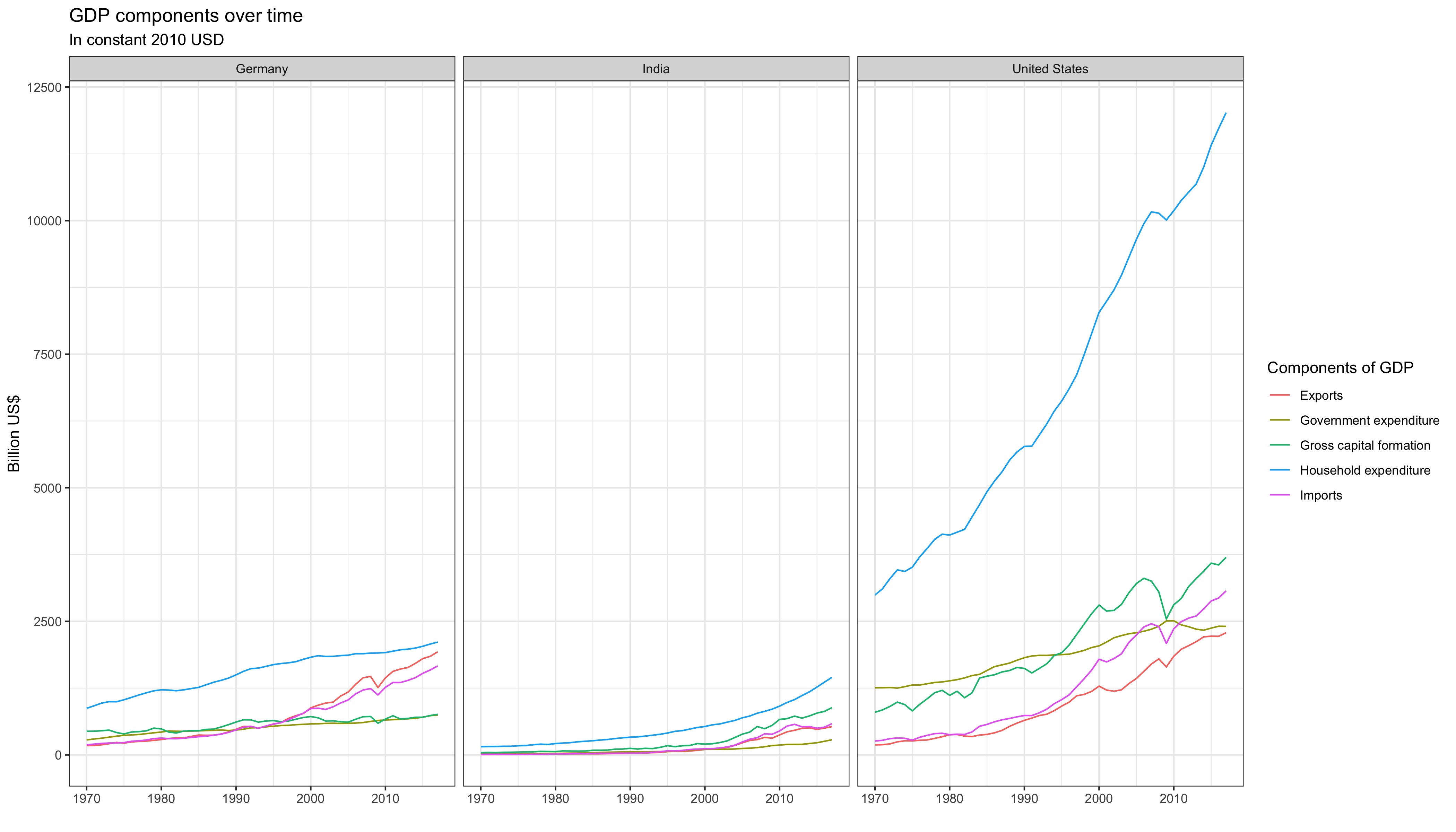
Plot 1
#Creating a set the country names and indicators needed for analysis
country_list <- c("United States", "India", "Germany")
gdp1_indicators = c("Gross capital formation", "Exports", "Government expenditure", "Household expenditure", "Imports")

#Creating line graph for germany, india, and united states along with their indicators
plot <- tidy_GDP_data %>%
  filter(Country %in% country_list, IndicatorName %in% gdp1_indicators) %>%
  ggplot(aes(x=Year, y=Value)) +
  #coloring the lines by the indicator names
  geom_line(aes(colour=IndicatorName)) +
  #making a separate plot for each country
  facet_wrap(~Country) +
  theme_bw() +
  scale_colour_discrete("Components of GDP") +
  labs(x="",
       y="Billion US$",
       title="GDP components over time",
       subtitle="In constant 2010 USD") +
  NULL
This plot depicts the % of government expenditure, gross capital formation, household expenditure, and net exports as a function of the respective country’s income. India - With the largest amount being spent on household expenditure, the gross capital formation is increasing while the household expenditure has started to decrease (considering that India is a developing country with low income, it is understandable that a huge chunk of income goes towards household expenses. However, the decrease in % spent on household income can be due to the improvement in the economy). Germany - They have relatively high exports when compared to India and US which can be allocated to the high exports from the automative industry (better technology). US - Just like Germany, the government expenditure and gross capital formation is at approximately 20% of income (however, India has grown to approximately 40%). Also, over the years the gross capital expenditure has taken over the government expenditure, showing that now people are investing more capital in the country than the governemnt. Nonetheless, we can not compare the expenditures of these countries in absolute terms as all these data points are a % of income and the income of each country varies.
Plot 2
gdp2_filter = c("Government expenditure", "Gross capital formation", "Household expenditure", "Exports", "Imports", "GDP")
gdp2_indicators = c("Government expenditure", "Gross capital formation", "Household expenditure", "Net Exports")

wide_GDP_data <- tidy_GDP_data %>%
  filter(Country %in% country_list, IndicatorName %in% gdp2_filter) %>%
 mutate(IndicatorName = case_when(
    IndicatorName == "Government expenditure" ~ "G",
    IndicatorName == "Gross capital formation" ~ "I",
    IndicatorName == "Household expenditure" ~ "C",
    TRUE ~ as.character(IndicatorName))) %>%
  pivot_wider(
    names_from=IndicatorName,
    values_from=Value) %>%
  mutate(
    NetExports=Exports-Imports,
    GDPManual=G+I+C+NetExports,
    C=C/GDPManual,
    I=I/GDPManual,
    G=G/GDPManual,
    NetExports=NetExports/GDPManual,
    GDPDifferencePct=(GDPManual-GDP)/GDP*100)


wide_GDP_data2<- wide_GDP_data %>%
  select(Country, Year, C, G, I, NetExports) %>%
  pivot_longer(cols=3:6, names_to='IndicatorName', values_to='Proportion') %>%
  mutate(IndicatorName = case_when(
    IndicatorName == "G" ~ "Government Expenditure",
    IndicatorName == "I" ~ "Gross capital formation",
    IndicatorName == "C" ~ "Household Expenditure",
    IndicatorName == "NetExport" ~ "Net Exports",
    TRUE ~ as.character(IndicatorName)))

plot <- wide_GDP_data2 %>%
  ggplot(aes(x=Year, y=Proportion)) +
  geom_line(aes(colour=IndicatorName)) +
  facet_wrap(~Country) +
  theme_bw() +
  theme(legend.title=element_blank()) +
  labs(x="",
       y="proportion",
       title="GDP and its breakdown at constant 2010 prices in US Dollars",
       caption="Source: United Nations, https://unstats.un.org/unsd/snaama/Downloads") +
  NULL